Building A Simple Malware Analysis Pipeline In The Homelab Pt - 1

About The Project

I wanted to further my malware analysis/reverse engineering skills and create a simple malware analysis pipeline. The pipeline I planned to build can be seen below.

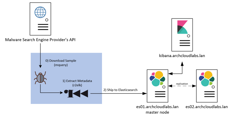
By collecting metadata about the binaries (imports/exports/pdbs/etc…) I can quickly filter and pivot on a subset of features that interest me. Over time it may be possible to enrich this data and have something really unique in the old homelab. However, before any analysis can begin I need to acquire samples.

Getting Samples from Malware Search Engines

Multiple malware research services exist that provide an avenue to search, download or upload malicious files to be executed in a sandbox environment. These providers typically provide API access to automate the tasks of interacting with their backend services. Of these providers, a handful offer free API access to some of these services. A subset of these providers include Malshare, Hybrid-Analysis, AV Caesar, VirusTotal, and (although currently under construction) Malwr.

It’s important to note that some of these services require a premium API key to access some of the services (such as downloading a sample). Out of the box, Malshare, AV Caesar and Hybrid-Analysis just require an account to be able to download samples. Hybrid-Analysis requires verification that you are indeed a researcher for some premium features, and VirusTotal offers a paid service to have access to their backend resources.

Each site provides extensive documentation on how to interact with their API. To consolidate time spent searching for samples, I wrote an API wrapper utility MQuery to query and download from multiple search engines.

MQuery & Provider APIs

MQuery checks which API keys currently exported as environment variables and will query those providers. Different providers treat what an “API request” looks like differently. For example, Malshare by default gives an end-user a thousand requests against their API regardless of the request. However, AV Caesar breaks down API usage into different buckets such as sample downloading, running samples in a sandbox environment, etc… keep this in mind when viewing output from the API info action within MQuery. Currently, mquery supports Malshare, Hybrid-Analysis, AV Caesar and VirusTotal public API endpoints. If you’re reading this and have access to a premium API key for Virus Total, consider testing and adding a feature to mquery to cover more of the premium features.

Downloading Samples

After running MQuery for about a month performing bulk daily binary pulls primarily from Malshare and Hybrid Analysis and After filtering down the downloaded samples a corpus of six thousand files was generated. It’s important to note that these files are from the API provider’s “daily feeds” and not individually pulled based on known “maliciousness”. While the files are likely malicious, anyone could upload a file to said provider.

Bulk Profiling Binaries

With a corpus of 6000 samples, data processing can begin! For the scope of this blog post, everything is going to be focused on the metadata extraction of binaries. Automation of the initial triage of binaries will occur via radare2 and the results will be stored in Elasticsearch. Over time, a robust database of artifacts will be gathered and perhaps assist in drawing interesting conclusions. While r2 may be a bit of overkill for some of the data that’s being extracted, understanding and fiddling with the API now may later lead to more advanced automation of binary triaging/analysis.

Initial triage of Binares with R2

Radare2 provides a robust shell to perform binary analysis. Almost all commands that can be executed from within the r2 shell can also be passed as command-line parameters. This provides an avenue for automating initial analysis. The i subset of r2 commands provides a way to gather information (imports, hashes, classes, strings, etc…).

The following r2 command will get general info and produce JSON output from a binary: r2 -c ij -q /usr/bin/ls. The command-line options are broken down as follows:

* -c: command to run
* i: give info about the binary
* j: display info in JSON
* -q: Quit r2 (do not return to the r2 shell)

After executing this command, r2 will return the following data:

{"core":{"type":"DYN (Shared object
file)","file":"/usr/bin/ls","fd":3,"size":137776,"humansz":"134.5K","iorw":false,"mode":"r-x","obsz":0,"block":256,"format":"elf64"},"bin":{"arch":"x86","baddr":0,"binsz":136048,"bintype":"elf","bits":64,"canary":true,"class":"ELF64","compiled":"","compiler":"GCC:
(GNU)
9.2.0","crypto":false,"dbg_file":"","endian":"little","havecode":true,"guid":"","intrp":"/lib64/ld-linux-x86-64.so.2","laddr":0,"lang":"c","linenum":false,"lsyms":false,"machine":"AMD
x86-64
architecture","maxopsz":16,"minopsz":1,"nx":true,"os":"linux","pcalign":0,"pic":true,"relocs":false,"relro":"full","rpath":"NONE","sanitiz":false,"static":false,"stripped":true,"subsys":"linux","va":true,"checksums":{}}}

The previous result was a bit hard to read. By piping this r2 command output into a Python JSON pretty print one-liner (python -m json.tool) a nicely formatted output is produced.

{
    "core": {
        "type": "DYN (Shared object file)",
            "file": "/usr/bin/ls",
            "fd": 3,
            "size": 137776,
            "humansz": "134.5K",
            "iorw": false,
            "mode": "r-x",
            "obsz": 0,
            "block":
                256,
            "format":
                "elf64"
    },
        "bin":
        {
            "arch":
                "x86",
            "baddr":
                0,
            "binsz":
                136048,
            "bintype":
                "elf",
            "bits":
                64,
            "canary":
                true,
            "class":
                "ELF64",
            "compiled":
                "",
            "compiler":
                "GCC:
                (GNU)
                9.2.0",
            "crypto":
                false,
            "dbg_file":
                "",
            "endian":
                "little",
            "havecode":
                true,
            "guid":
                "",
            "intrp":
                "/lib64/ld-linux-x86-64.so.2",
            "laddr":
                0,
            "lang":
                "c",
            "linenum":
                false,
            "lsyms":
                false,
            "machine":
                "AMD
                x86-64
                architecture",
            "maxopsz":
                16,
            "minopsz":
                1,
            "nx":
                true,
            "os":
                "linux",
            "pcalign":
                0,
            "pic":
                true,
            "relocs":
                false,
            "relro":
                "full",
            "rpath":
                "NONE",
            "sanitiz":
                false,
            "static":
                false,
            "stripped":
                true,
            "subsys":
                "linux",
            "va":
                true,
            "checksums":
            {}
        }
}

Excellent! This is much easier to read and see what would be beneficial to parse. Some additional commands the r2 enthusiast/analyst may find interesting are as follows:

• Show hashes: r2 -c itj -q /usr/bin/ls

• Show linked libraries (can be verbose): r2 -c ilj -q /usr/bin/ls

• Show all info (very verbose): r2 -c iaj -q /usr/bin/ls

These commands provide individual JSON objects and can later be used to ingest into other tools or databases such as Elasticsearch.

Storing The Results

An Overly Simplified Introduction on Elasticsearch

Elasticsearch is a NoSQL database that provides significant flexibility on how end users can store and search their data. There are several ways to configure and deploy Elasticsearch to aid in ingest/horizontal scalability. One of the main considerations when creating an index (database for the RDBMS users) is how many shards to create. Elasticsearch, The Definitive Guide defines a shard as “a low-level worker unit that holds just a slice of all data in the index”. The number of primary and replica shards created will also reflect on how robust to failure your cluster is for a given index.

After an index has been created the number of shards cannot be updated. You can create a new index and reingest data from other indexes into it. Depending on the amount of data you have this may be a large ordeal. However, this isn’t a production environment, so using one primary shard with no replica shards (as it’s a stand-alone Docker container) will suffice for now. For more on Elasticsearch, and how it works under the hood, I highly recommend Elasticsearch, The Definitive Guide. Be aware some large changes came with 7.X releases. Checking the release notes of 7.X should provide sufficient information to bridge the knowledge gap between releases.

Deploying Elasticsearch & Kibana

The installation of Elasticsearch is outside the scope of this blog post. There are several posts documenting a typical ELK deployment. Logstash is not being used for the time being as data is being extracted and ingested directly into Elasticsearch via r2 and additional manipulation is not needed server-side. For now, leveraging r2 to do the heavy work will be just fine. For an in-depth guide on how to install the entire ELK stack, I recommend the official documentation. I will be leveraging Elastic co’s Docker image for initial prototyping.

Execute the following command to have an Elasticsearch database up and running:

docker run --name elasticsearch -p 127.0.0.1:9200:9200 -e "discovery.type=single-node" docker.elastic.co/elasticsearch/elasticsearch:7.3.1

Ensuring Elasticsearch is running can be accomplished via docker ps or execute: curl 127.0.0.1:9200. If the curl command was successful, the output below should be produced.

{
    "name" : "hostmachine",
        "cluster_name" : "docker-cluster",
        "cluster_uuid" : "CkXwypRUQquT7CRk_eKfcg",
        "version" : {
            "number" : "7.3.1",
            "build_flavor" : "default",
            "build_type" : "docker",
            "build_hash" : "4749ba6",
            "build_date" : "2019-08-19T20:19:25.651794Z",
            "build_snapshot" : false,
            "lucene_version" : "8.1.0",
            "minimum_wire_compatibility_version" :
                "6.8.0",
            "minimum_index_compatibility_version"
                : "6.0.0-beta1"
        },
        "tagline" : "You Know, for Search"
}

It is possible to perform headless queries via curl, but it’s less than desirable. Kibana enables the end-user to create robust dashboards and leverage a powerful search capability that can lead to discovering new insights about our data. To deploy Kibana alongside the Elasticsearch container, execute the following: docker run --link elasticsearch -p 127.0.0.1:5601:5601 docker.elastic.co/kibana/kibana:7.3.1

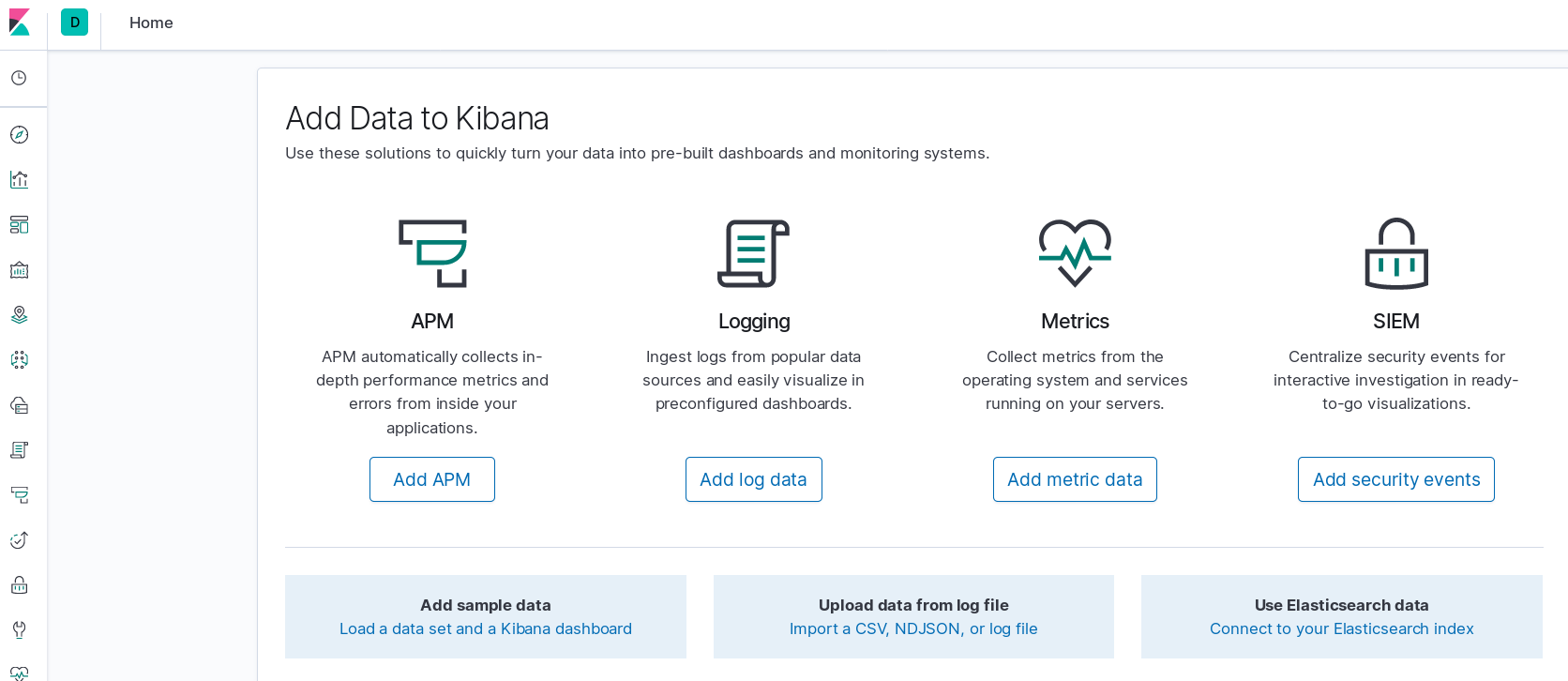
At this point, you should be able to visit http://127.0.0.1:5601 and see the Kibana homepage (example shown below).

If something goes awry, likely Kibana cannot talk to Elasticsearch. By default, the Docker Kibana container will try to connect to Elasticsearch via a hostname of “elasticsearch”. Be sure to add the --name switch when running the Elasticsearch Docker run command. For more on Kibana and Docker, see here.

Now that Elasticsearch and Kibana are running, data ingestion can begin.

Storing R2’s Output

By leveraging the previous r2 triage command’s stdout to curl, results can be ingested directly into Elasticsearch. The -d @- command-line options below specifies the body of the POST request to be based on stdin The entire command can be seen here: r2 -q -c iaj /usr/bin/ls | curl -XPOST -H "Content-Type: application/json" http://127.0.0.1:9200/test/_doc -d @-

If everything worked correctly, data should be made available via Kibana. An initial peak at what was just ingested shows metadata from one of the binaries from the sample set.

Opening Kibana and creating a search index will result in something similar to the image below:

Limitations of Elasticsearch with Nested Data

The data is now in Elasticsearch and is searchable, but there’s an issue. The small triangles in the previous image indicate a warning from Kibana stating that “objects in arrays are not well supported”. The nested data is less than desirable for searching.

Elasticsearch’s Lucene based search does not perform well with nested data. The previous section demonstrated how to store r2 output into Elasticsearch for searching with a single bash one-liner. Unfortunately, some of these fields resulted in nested objects. While it’s possible to query for specific fields, Elasticsearch’s performance may be impacted.

This is a test-bed for experimentation with a small dataset so perhaps waiting an extra second or two isn’t the end of the world . However, In a production environment this is less than ideal. By leveraging r2’s Python bindings and performing additional data manipulation the nested JSON objects can be avoided and made into something that will make our searchers easier.

Breaking Out Nested Data

By breaking out JSON objects into individual fields the nested data issue can be avoided. This was accomplished via r2 Python bindings. Multiple r2 commands can be combined into a single JSON data object via Python before Elasticsearch ingestion. To accomplish this I wrote r2elk. R2elk performs the same commands previously discussed, but populates a dictionary with metadata parsed from a binary and enables the end-user to then perform an HTTP(s) POST to an endpoint or simply print the data to stdout. This enables cleaner data ingestion into Elasticsearch while still using the underlying r2 framework.

Listing Imports & Exports

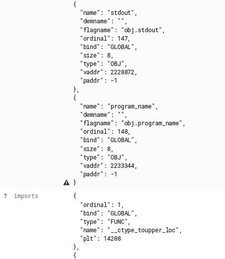
Originally, each function import/export was treated as a stand-alone field. This approach results in a significant amount of fields being generated, especially with larger libraries. This functionality remains within r2elk, but the methods are not called by default. To support indexes with over 1000 fields within a single document, the index field limits must be updated. See this link for additional details. The image below shows the verbosity of this approach and how quickly you can approach the default 1000 field limit of an Elasticsearch index.

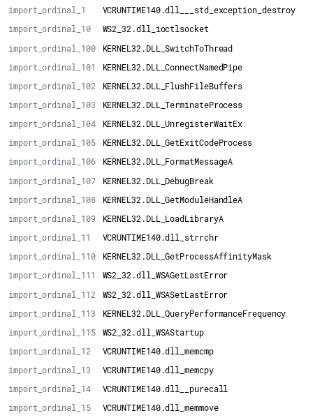
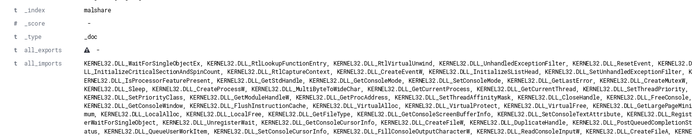
By default, a single field of “imports” will map to a comma-delimited field which contains all imports. An example of an import field from an individual document ingested into Elasticsearch is shown below.

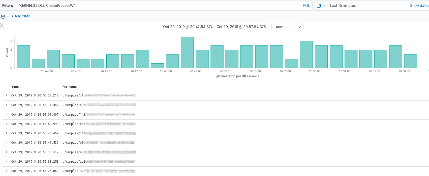
While messy, if searching for specific DLL usage across a data set, meaningful results can be obtained by filtering on additional document attributes such as file name. The example below shows the file name of executables that include the function “CreateProcessW”.

If an end-user would prefer to change the triage to produce multiple fields of imports/exports per-binary, the README within the r2elk repo explains how to modify the run_triage function to produce said output.

Getting to Know The Data

With data coming in via r2elk, it is time to take a look at what Kibana raw search can provide.

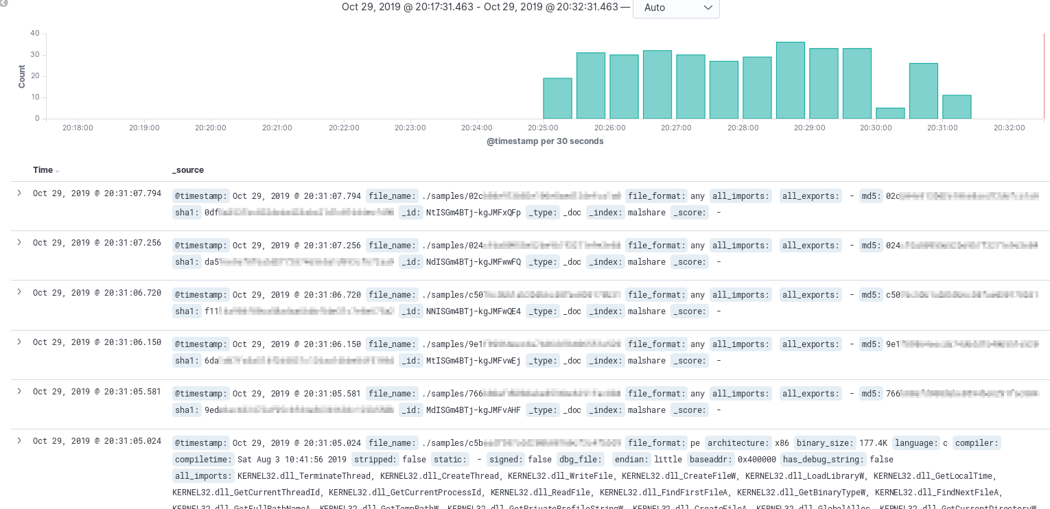
The image above shows that the first few records are severely lacking data, oh no! What could this mean? Maybe there’s a problem with the downloader? Could the file be corrupt? Well, the file path is there, so let’s dive in and see what the issue is! In this scenario, there was a file that wasn’t a PE or ELF so the additional fields were not attempted to parse. If you have honeypots that are collecting a lot of initial downloader scripts you’re likely to run across a similar scenario. The last document shown appears to have parsed out nicely and actually has quite a few imports.

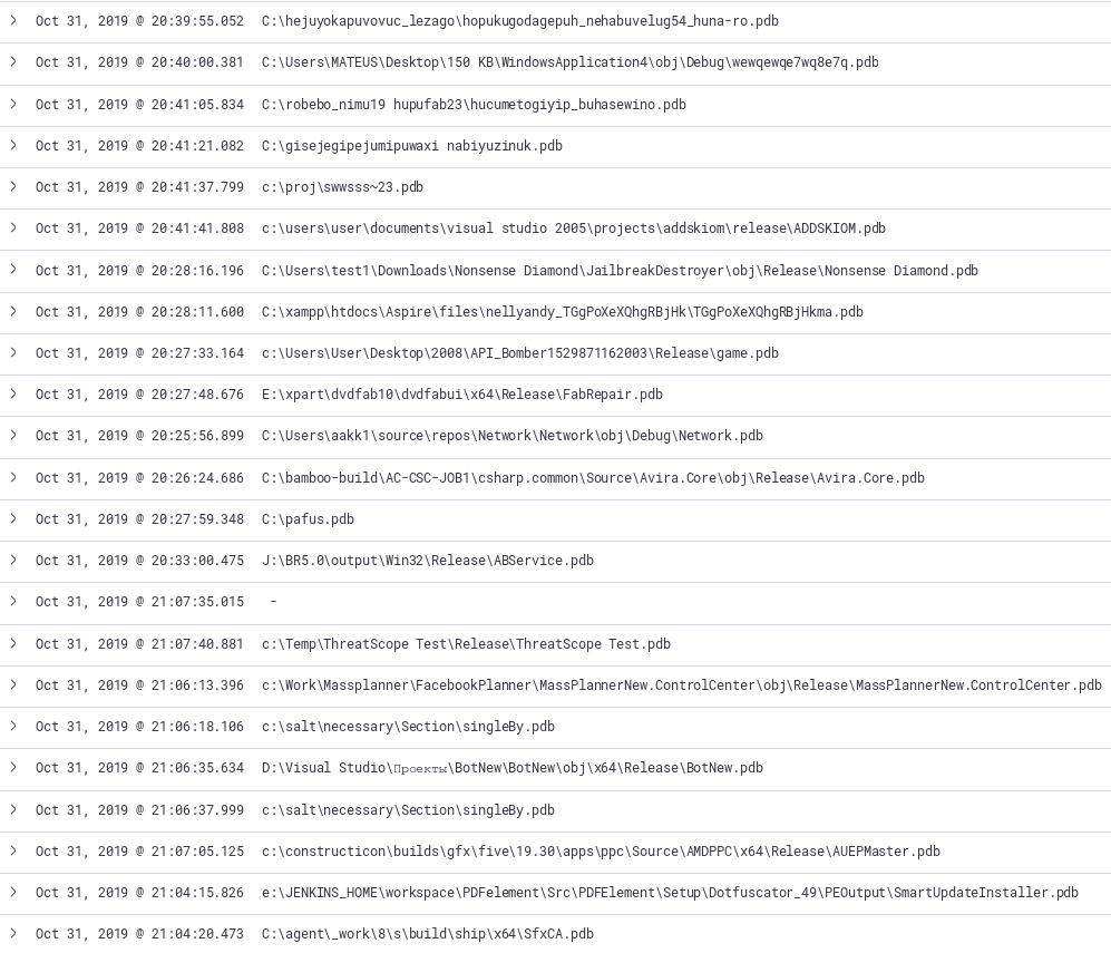
Inspired from this FireEye blog post, PDB debug strings are interesting artifacts of the development environment is presented to the analyst. By looking across a large dataset further links may be drawn on similar samples. Leveraging filters in Kibana, we can filter on samples that have PDB files extracted and observe anything that might be of interest. The image below shows a couple interesting artifacts from the sample set having words such as “API Bomber” or “BotNew”. This query can also act as a jumping off point to start manually samples that sound interesting.

Example Visualizations

After running r2elk through all 6k samples I have a nice corpus of data to build visualizations and gain insight from. Initially, I filtered for just DLLs files and created a pie graph to see top functions. The image below shows a nice breakdown of what exists in my dataset.

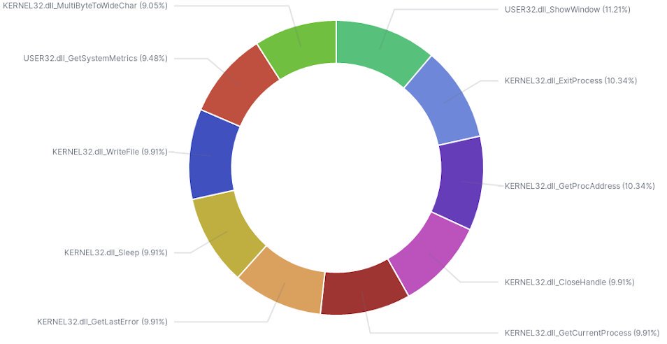
While not entirely helpful on a larger scale, understanding top DLL usage in a subset of similar samples may lead to better strategies for static analysis.

Next Steps

Now that a rudimentary way to ingest, extract metadata, and create some quick visualizations has been created it’s time to flush out the ingestion! The next post will dive into Yara integration to further enrich the metadata.

I hope you found the content entertaining and informative. Thank you for taking the time to read this.